The internal rates of return (IRR) for our model of a typical Haynesville dry gas shale well is in the low teens at today’s gas prices. That is a low return compared to the liquids rich plays that producers are concentrating on these days. The economics of shale well production are calculated the same way for liquid shale plays – there is just more uplift from the higher priced liquids output. And natural gas output continues to surge with associated gas from the liquid wells. Today we complete our analysis of shale production economics.
Recap And Spreadsheet Model Download
In the first episode in this series (see Drilling) we discussed “unconventional resources” and conventional hydrocarbon drilling then reviewed the technologies developed by the late George Mitchell and his team to produce unconventional shale resources. In the second episode (see Shale Production Economics – Part 2 – Drilling and Completion Costs) we introduced the eight input factors for our model of production economics and provided example values for drilling and completion costs. In part 3 we explained four techniques to forecast initial production (IP), decline rate and estimated ultimate recovery (EUR) for a shale gas well (see Shale Production Economics Part 3 – Estimating Well Production). Unconventional shale wells are characterized by high IP rates and steep decline rates but the high early production rate provides drillers with a rapid return on their investment, which makes these plays so economically attractive. In episode four we looked at variable production costs for a shale gas well – including lease operations, transportation to market, royalties and taxes (see Variable Cost and Net Present Value). In episode 5 we took you through the input variables for our model well (see Shale Gas Production Economics Spreadsheet Model and Inputs). We also provided a downloadable spreadsheet for you to test out the sensitivities of the production and cost variables for a Haynesville shale gas well. You can still access the download here. [To download the file, you must be logged in as a registered RBN Backstage Pass subscriber. If you are not yet a subscriber, you can sign up here.] If you are a subscriber and you have trouble downloading the file (usually some firewall issue), then let us know at [email protected] and we will send you a copy. Please note that the spreadsheet model is provided as an example, not a definitive well economics predictor. Don’t call us up if your production well does not achieve the rate of return you expected. There are some comments from members about the handling of lease costs below the episode 5 blog. [Note that our model example is ‘half cycle’ economics. That is, we don’t include lease acquisition costs in our calculations. Thus we are showing the incremental return from drilling the well, not the total return. This approach is relevant when measuring the lilklihood that producers will drill in existing plays like Haynesville where many leases have already been obtained and are held by production on the lease. Also note that depreciation is irrelevant in our calculations since we are computing before tax returns.]
In this series we are modeling the economics of shale production with reference to a specific example – the Haynesville Shale. We use the Haynesville because it is a dry gas formation, meaning that only natural gas (“mostly methane”) is produced. That allows us to model the production economics without having to delve into the complexities associated with wet gas (including NGL) or combined crude and gas liquids. These liquid hydrocarbons are, of course very important to many US shale plays today, but once you understand the economic returns on a dry gas well then the liquids produced from wet gas or oil wells can be viewed as an additional uplift dimension to the basic model.
Model Outputs
This time we take you through the model outputs. In order to do that, it probably makes sense for you to download the sheet as instructed above, so that you can follow along in Excel. We went through the input variables in the sheet last time and we reproduce that graphic first for reference (see Figure 1 below). Go back to the previous episode for further detail on each input. The input cells on the graphic are those with colored boxes and the rows and columns marked are the same as those in the spreadsheet version.
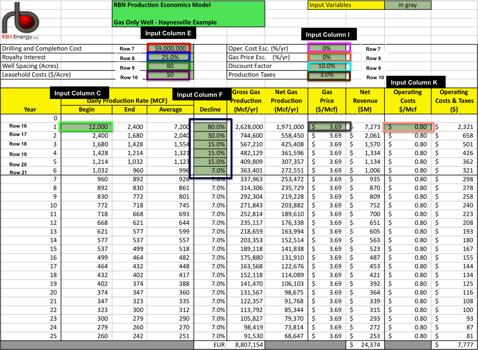
Figure 1 Source: RBN Energy (Click to Enlaerge)
Figure 2 below is the “output” area of the spreadsheet model. The cells in this graphic are located to the right of the input area on the spreadsheet – we just separated them in this blog to make things more legible. As with the input variables, we marked the row and column numbers of the spreadsheet cells that we will refer to. The data that we are using for this explanation starts with the assumption that the input variables are set to their defaults in the download sheet – the same values you see in Figures 1 and 2.